Calculating Heat Flow and Thermal Bridges
The appendix contains the most important parameters for constructional thermal insulation at a glance.

Basic Definitions
Thermal conductivity quantifies the ability of a material to transmit heat in terms of energy by unit thickness and by degree of temperature difference, see Table 4.

Table 4: thermal conductivity of a range of materials
Thermal resistance
The thermal resistance R is the resistance to heat flow with K temperature difference across one m2 and is based on the conductivity λ. R is calculated as the thickness (t) of the material divided by its thermal conductivity:
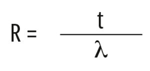
λ: Thermal conductivity in W/(mK)
t: Material thickness in m
This calculation of the R-value can also be performed for multilayer components:
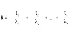

Figure 26: A representation of a wall construction, to define the R value by the thickness of the layers and the corresponding λ value.
The U-value, or thermal transmission coefficient, quantifies the heat flow through a building construction by the degree temperature difference across it. It is calculated as the reciprocal value of the sum of the thermal resistances and the surface resistances Rsi and Rse:
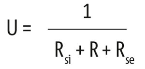
The U-value describes one dimensional heat flow per square metre of component per degree temperature differential across it, which is needed to calculate the energy loss of areas of the same assembly. U-value is not applicable to areas of thermal bridges, such as that shown in Figure 27. For more information about Basic Definitions, see Apendix 4.3.

Figure 27: Representation of a temperature profile through a wall. The slope of the temperature profile is defined by the thickness of the layers and the corresponding R value. At the surfaces the surface resistances Rsi and Rse also take effect. On the right hand side you can see how the temperature profile between the different layers is calculated.
Consideration of lateral Heat Flow
Figure 28 illustrates several important concepts using the example of a slab, such as a balcony, penetrating a wall and therefore the insulation layer:
- Heat will flow laterally to the easiest path through the assembly (i.e. the slab).
- The planar heat flow (U) is the heat flow through an assembly without thermal anomalies. The linear thermal transmittance is the additional heat flow with the thermal anomaly due to lateral heat flow as shown in Figure 28.
- One can view the influence of the thermal bridge as being an additional heat loss due to the slab (the yellow area under curve on the graph) that is added to the heat loss of the wall without the slab (the blue area of the graph).

Figure 28: Pattern of heat flow through a building envelope with materials that allow lateral heat flow to a thermal bridge.
Recognizing that the heat flow through a thermal bridge can be added to the heat flow through a planar building assembly provides a method of accounting for thermal bridges that cannot really be addressed by the "parallel path" method of the equations in Chapter 4.3. This is particularly true when the power of computer modelling can be used to determine the heat flow attributable to specific types of thermal bridges. It has proven useful to classify thermal bridges by how one would add them up: Figure 29 illustrates an example of using computer modelling to determine the Ψ value of a linear thermal bridge, in this example a slab penetrating a wall. One creates two "models" with the same width and height:
- The impact of small, frequent and distributed bridging elements (e.g. brick ties or Z-spacers carrying cladding as seen in Figure 29 on the following page) are generally best handled by adding their thermal influence to U-value (W/(m²K) for the assembly. These are repeating thermal bridges, and they are included in the U-value calculation.
- The heat transfer associated with linear elements (e.g. slab edges, corners, roof/wall intersections, window wall interfaces etc.) can be handled by determining the Linear Heat Transmittance coefficient W/(mK). The Greek letter Psi (Ψ) is conventionally used to represent a linear transmittance.
- The heat transfer associated with intermittent or singular elements (e.g. beams or other projecting structural elements) can be handled by determining the Point Heat Transmission coefficient (W/K)). The Greek letter Chi (χ) is conventionally used to represent a point transmittance.
1. The wall without the slab but with the frequent and distributed bridging elements (the Z-spacers in this case) that you would want to include in the U-value. The program provides the steady state heat flow for the assembly (Q).
2. The assembly including the slab. The program provides the steady state heat flow for the combined assembly (Q).

Figure 29: Example of process of determining the linear transmittance of a slab penetrating a wall.
The difference in heat flow between the two models divided by the width of the modelled sections is the linear transmittance or Ψ for slab. This value is effectively the area under the yellow curve in Figure 28.
A similar process can be used to calculate the point transmittance of a beam penetrating a wall.
Linear and point transmittances can be determined by two or three dimensional thermal modelling for specific details. Using this concept, the total heat flow through a wall, roof or floor with linear and point thermal bridges is calculated by adding the heat flow through the thermal bridges to that through the clear field of the assembly.
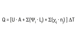
where
U is the "clear wall" assembly heat transmittance (including the impact of frequent and distributed bridging elements)
A is the area of the assembly, including all details in the analysis area
Ψi is the linear thermal transmittance value of detail "i"
Li is the total length of the linear detail "i" in the analysis area
χj is the point heat transmittance value of detail "j"
n is the number of point thermal bridges of type "j" in the analysis area
The examples in Chapter 3 and 4 use this method of calculation.